Model

Definitions

The sets and their associated parameters are shown in Table 1. We elaborate on a few aspects of this model. If the working capacity at an airport is reached, then a plane will wait for an open slot. Once the airplane starts processing, it will need a fixed amount of processing time \(\processtime{p}\), regardless of whether cargo is being loaded or unloaded. As in [2], we impose two deadlines: one is a soft deadline \(\softdeadline{c}\) by which the cargo is expected to be delivered, and one is a hard deadline \(\harddeadline{c}\) after which the delivery is considered missed and no longer useful.

Table 1 Sets and parameters

Set	Description	Associated Parameters
\(\Airports\)	Airports	For airport \(a \in Airports\): Working capacity (number of planes that can be processed at same time): \(\workingcapactity{a}\)
\(\Routes\)	Routes between airports	For route \(r \in \Routes \subseteq \Airports \times \Airports\): Cost of flying route by airplane \(p \in \Airplanes\): \(\routecost{r}{p}\) Time required for airplane \(p \in \Airplanes\) to fly route: \(\routetime{r}{p}\) Start/end airports: \(\routestart{r},\routeend{r} \in \Airports\) Note: Routes are directed, i.e., the route between airports \(a_{1}\) and \(a_{2}\) is distinct from the route from \(a_{2}\) to \(a_{1}\).
\(\Airplanes\)	Airplane	For airplane \(p \in \Airplanes\): Cargo weight capacity: \(\weightcapacity{p}\) Time to process: \(\processtime{p}\) In practice, we will have a small number of airplane types which will have shared parameterizations. We leave this as an implementation detail.
\(\Cargos\)	Cargo items	For cargo item \(c \in \Cargos\): Weight: \(\cargoweight{c} \in \Reals\) Location/destination airports: \(\cargoloc{c},\cargodest{c} \in \Airports\) Target delivery time: \(\softdeadline{c}\) Delivery deadline: \(\harddeadline{c}\)

Dynamic Features

We start by providing a list of variables. For brevity, we only identify key variables rather than provide an exhaustive list. Given airplane \(p \in \Airplanes\) and airport \(a \in \Airports\), Table 2 defines variables and sets that reflect the environment state at time \(t\).

Table 2 State

Variable / Set	Description
\(\currentairport{p}{t} \in \Airports\)	The current location of airplane \(p\).
\(\AvailableRoutes{t} \subseteq \Routes\)	Set of available routes.
\(\CargoOnPlane{p}{t} \subseteq \Cargos\)	The set of cargo loaded on airplane \(p\)
\(\CargoAtAirport{a}{t} \subseteq \Cargos\)	The set of cargo stored at airport \(a\)
\(\AirplanesAtAirport{a}{t} \subseteq \Airplanes\)	The set of planes processing at airport \(a\)

The following dynamic events may occur:

• A new cargo order is added to set \(C\).

• Route \(r \in R\) becomes temporarily unavailable for landing or takeoff (e.g., due to weather). Flights already en-route will still complete the flight to the destination.

The available actions for each agent are shown Table 3. Note that actions may become invalid as the state of the model evolves (for example an airplane’s destination may become unreachable).

Table 3 Actions for airplane \(p \in \Airplanes\) at time \(t\)

Action	Description
\(\process{p}\)	Boolean indicating whether airplane should refuel and load/unload cargo when landed.
\(\cargotoload{p} \subseteq \CargoAtAirport{\currentairport{p}{t}}{t}\)	Boolean indicating whether or not route \(r\) is available.
\(\cargotounload{p} \subseteq \CargoOnPlane{p}{t}\)	The set of cargo unload from the airplane.
\(destination\) \(\in \{ a_2 \in \Airports | (\currentairport{p}{t}, a_2) \in \AvailableRoutes{t} \}\)	The next destination of the airplane.

Airplane State Machine

A state machine for the airplane is shown in Fig. 1 (see a list of airplane states with descriptions). Airplanes must process at least once after landing before they can before they are fully fueled and ready to take off. Although we do not explicitly model fuel usage, the processing state introduces a wait typically needed for refueling and other maintenance. The agent may choose to load/unload cargo during processing, or may simply process the airplane without moving cargo. While the cargo is being loaded, it will be removed from the airport cargo set during processing, and then added to the airplane cargo set when finished. A similar process is followed for unloading cargo. Once ready for takeoff, the agent may choose to re-process the plane so that cargo can be loaded/unloaded (perhaps in response to recent events), or may specify a route for takeoff. The airplane will only take off if the route is available, i.e., if a random event has not taken the route offline. While in-flight, the airplane moves at a uniform rate along the route, set according to the flight time for that plane on the given route. The agent cannot issue any actions during the flight. Once it reaches an airport, the airplane will land and return to a waiting state pending further action by the agent.

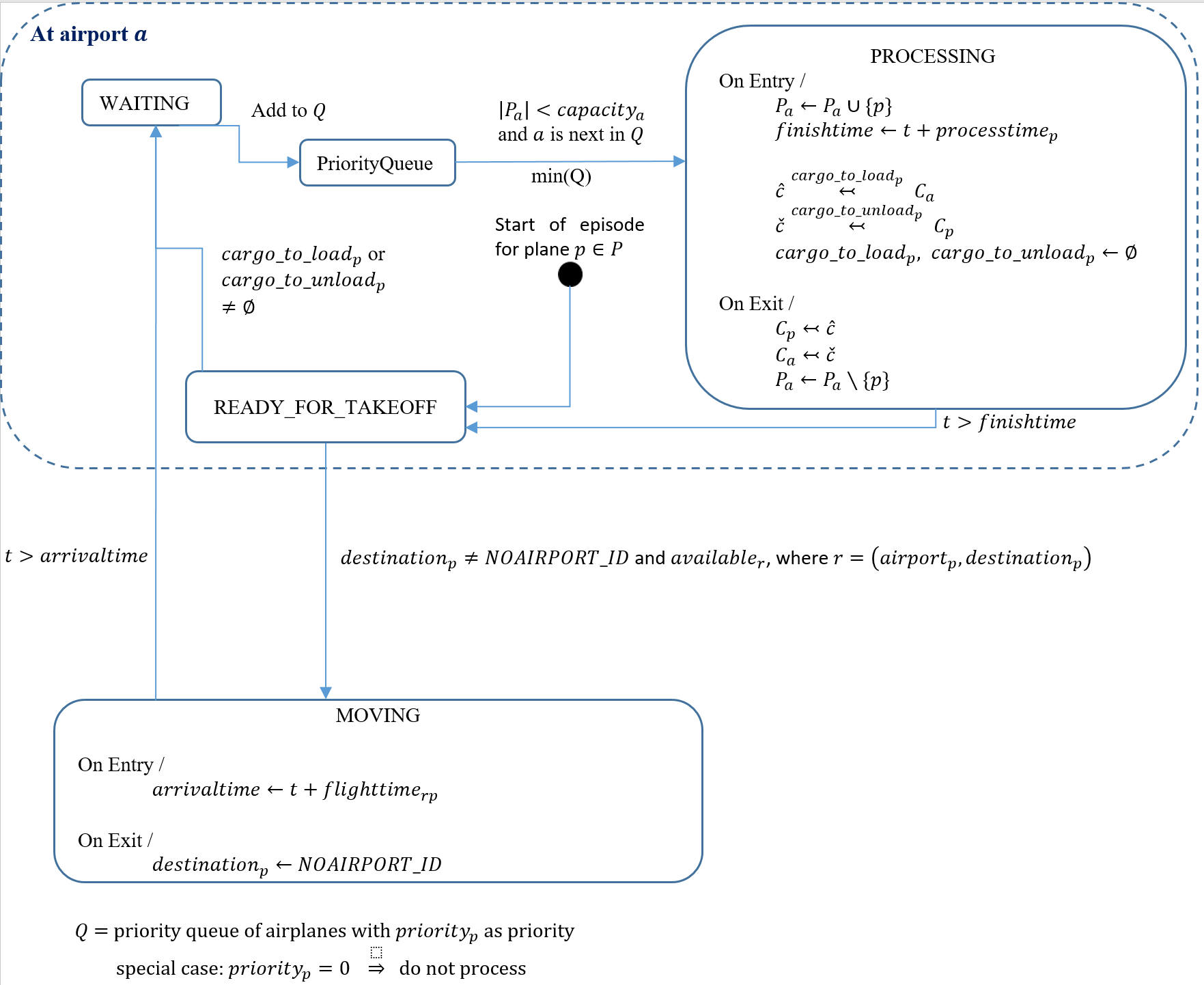
Fig. 1 Airplane state machine. Time parameters are omitted from events for clarity. The transition labels indicate the condition required for the transition to occur. State transitions are evaluated at each time step. The notation \(\mathbf{A} \stackrel{\mathbf{B}}{\leftarrowtail} \mathbf{C}\) indicates that the elements in set \(\mathbf{B}\) are removed from set \(\mathbf{C}\) and added to set \(\mathbf{A}\) (if \(\mathbf{B}\) is omitted, all elements are moved from set \(\mathbf{C}\) to \(\mathbf{A}\)).

Metrics

We base the score and reward on three raw metrics:

(1)\[\missed = \sum_{c \in \Cargos} \Indicator{\actualdelivery{c} > \harddeadline{c}},\]

(2)\[\begin{split}\lateness{c} =& \max \left\{ 0, \actualdelivery{c} - \softdeadline{c} \right\} \\ &\qquad * \,\, \Indicator{\actualdelivery{c} \leq \harddeadline{c}},\end{split}\]

(3)\[\flightcost{p} = \sum_{r \in \Routes} \left( \routecost{r}{p} * \numflights{r}{p} \right),\]

where \(\Indicator{\cdot}\) is the indicator function, \(\actualdelivery{c}\) is the actual time when the cargo is delivered (or \(\infty\) if the delivery never occured), and \(\numflights{r}{p}\) is the number of flights by plane \(p\) over route \(r\). The number of missed deliveries is captured by (1). For deliveries that are not missed, (2) indicates the amount of time by which these deliveries miss the delivery deadline. The cost incurred by airplane \(p\) flying routes during the course of the episode is identified by (3). We note that although the cost may be primarily driven by fuel usage, it can also quantify other costs.

In order to encourage more uniformity across scenarios, we derive two scaled metrics. First, we scale the lateness so that it’s value will range between 0 and 1:

(4)\[\scaledlateness = \sum_{c \in \Cargos} \frac{\lateness{c}}{\harddeadline{c} - \softdeadline{c}}\]

Second, we scale the flight costs of each airplane against the diameter of the route map graph, the number of cargo generated \(\totalcargo\), and the capacity of the airplane. Specifically, the total scaled flight cost over all planes is defined as

(5)\[\scaledflightcost = \sum_{p \in \Airplanes} \frac{\flightcost{p} * \routemapdiameter{p}} {\weightcapacity{p} * \totalcargo},\]

where \(\routemapdiameter{p}\) is the diameter of the largest connected component of airplane \(p\)’s route map.